3. User guide

3.1. Densities

Pypmc revolves around adapting mixture densities of the form

\[q(x) = \sum_{j=1}^K \alpha_j q_j(x), \: \sum_{j=1}^K \alpha_j = 1\]

where each component \(q_j\) is either a Gaussian

\[q_j(x) = \mathcal{N}(x | \mu_j, \Sigma_j)\]

\[q_j(x) = \mathcal{T}(x | \mu_j, \Sigma_j, \nu) \,.\]

The free parameters of the mixture density, \(\theta\), are the component weights \(\alpha_j\), the means \(\mu_j\), the covariances \(\Sigma_j\) and in case \(q_j = \mathcal{T}\) the degree of freedom \(\nu_j\) for \(j=1 \dots K\).

3.1.1. Component density

The two densities — Gauss and Student’s t — supported by pypmc come in two variants whose methods have identical names but differ in their arguments. The standard classes are Gauss and StudentT:

mean = np.zeros(2)
sigma = np.array([[ 0.1,  -0.001],
                    [-0.001, 0.02]])
dof = 5.
gauss = pypmc.density.gauss.Gauss(mean, sigma)
student_t = pypmc.density.student_t.StudentT(mean, sigma, dof)

# density at (1, 1)
f = gauss.evaluate(np.ones(2))

# draw sample from density
x = gauss.propose()

For the use as proposal densities in Markov chains (see below), there are also local variants whose mean can be varied in each call to evaluate or propose. LocalGauss and LocalStudentT don’t take the mean argument in the constructor. To reproduce the previous results, one would do:

local_gauss = pypmc.density.gauss.LocalGauss(sigma)
f = local_gauss.evaluate(mean, np.ones(2))
x = local_gauss.propose(mean)

3.1.2. Mixture density

Mixture densities are represented by MixtureDensity. One can create a mixture density from a list of arbitrary component densities and weights. However, usually all one needs are the convenience shortcuts to create mixtures of Gaussians and Student’s from means and covariances. For example, for two components with weight 60% and 40%:

from pypmc.density.mixture import create_gaussian_mixture, create_t_mixture
weights = np.array([0.6, 0.4])
means = [np.zeros(D), np.ones(D)]
covariances = [np.eye(D), np.eye(D)]
gauss_mixture = create_gaussian_mixture(means, covariances, weights)

dofs = [13, 17]
mixture = create_t_mixture(means, covariances, dofs, weights)

The most common interaction pattern with a mixture density requires only a few attributes and methods:

gauss_mixture.evaluate(np.zeros(D))
samples = gauss_mixture.propose(N=500)
D = gauss_mixture.dim
first_component = gauss_mixture.components[0]
second_weight = gauss_mixture.weight[1]

3.2. Indicator function

The indicator function \(\mathbf{1}_V\) can be used to limit the support of the target density to the volume \(V\) in the samplers discussed below. It is defined as

\[\begin{split}\mathbf{1}_{V} (x) = \begin{cases} 1, x \in V \\ 0, {\rm else} \end{cases}\end{split}\]

The indicator module provides indicator functions for a ball and a hyperrectangle in \(D\) dimensions. The indicator function can be merged with the (unbounded) target density such that the wrapper calls the target density only if the parameter vector is in V and returns \(\log(0)= -\infty\) otherwise:

from pypmc.tools.indicator import \
     merge_function_with_indicator

def target_density(x):
    # define unbounded density on log scale

# define indicator
ind_lower = [p.range_min for p in priors]
ind_upper = [p.range_max for p in priors]
ind = pypmc.tools.indicator.hyperrectangle(ind_lower, ind_upper)

# merge with indicator
log_target = merge_function_with_indicator(target_density, ind, -np.inf)

3.3. Markov chain

3.3.1. Initialization

We provide a generic implementation of adaptive local-random-walk MCMC [HST01] featuring Gauss and Student’s t local proposals. To create a MarkovChain, one needs three ingredients:

Evaluate the target density on the log scale.
A local proposal density.
A valid initial point.

For example:

import pypmc.density.student_t.LocalStudentT
import pypmc.sampler.markov_chain.AdaptiveMarkovChain

# unit gaussian, unnormalized
def log_target(x):
  return -0.5 * x.dot(x)

prop = LocalStudentT(prop_sigma, prop_dof)

start = np.array([-2., 10.])
mc = AdaptiveMarkovChain(log_target, prop, start)

The initial proposal covariance should be chosen similar to the target’s covariance, but scaled to yield an acceptance rate in the range of 20%. For a Gaussian target and a Gaussian proposal in \(D\) dimensions, the scaling should be \(2.38^2/D\).

In order to constrain the support of the target in a simple way, one can pass an indicator function to the constructor using the keyword argument ind=indicator. Then any proposed point is first checked to lie in the support; i.e., if indicator(x) == True. Only then is the target density called. This leads to significant speed-ups if the mass of the target density is close to a boundary, and its evaluation is slow.

3.3.2. Adaptation

The prototypical use is to run the chain for a number of iterations until it finds the bulk of the distribution, and to discard these samples as burn-in or warm-up. Then the samples can be used to tune the proposal covariance:

mc.run(10**4)
mc.clear()

# run 100,000 steps adapting the proposal every 500 steps
# hereby save the accept count which is returned by mc.run
accept_count = 0
for i in range(200):
accept_count += mc.run(500)
mc.adapt()

Note that the proposal can be tuned continously so the Markov property is lost but the samples are still asymptotically distributed according to the target; i.e., there is no need to fix the proposal to generate valid samples.

The parameters like the desired minimum and maximum acceptance rate can be set via set_adapt_params.

3.4. Importance sampling

3.4.1. Standard

The standard ImportanceSampler implements serial importance sampling to compute the expectation of some function \(f\) under the target \(P\) as

\[E_P[f] = \int dx P(x) f(x) \approx \frac{1}{N} \sum_{i=1}^N P(x_i) / q(x_i) f(x_i)=\frac{1}{N} \sum_{i=1}^N w_i f(x_i), x \sim q,\]

where \(w_i\) is the importance weight and \(q\) is the proposal density.

To start, one only needs the target density \(P\) defined by a function that computes \(log(P(x))\) for an input vector \(x\), and similarly for \(q\):

import pypmc.sampler.importance_sampling.ImportanceSampler

sampler = ImportanceSampler(log_target, log_proposal)

Optionally, the sampler accepts an indicator; see Indicator function. What to do with sampler? Run it:

sampler.run(N=500)

to draw 500 samples. If the proposal is a MixtureDensity and the option trace_sort=True, then run returns the generating component for each sample.

The samples and weights are stored in two history objects:

samples = sampler.samples[-1]
weights = sampler.weights[-1]

Note that a History object can contain the output of several runs, the last one is available as history[-1].

The samples are ordered according to the generating component if trace_sort=True.

3.4.2. Deterministic mixture

If weighted samples from the same target but different proposal densities are available, the weights can be combined in a clever way as though they were drawn from the mixture of individual proposals [Cor+12]. This preserves the unbiasedness of the fundamental estimate of importance sampling. The motivation to combine multiple proposals is to improve the variance of the estimator by reducing the effect of outliers; i.e., samples with very large weights in the tails of \(q\). For proposals \(\{q_l: l=1 \dots T\}\) and \(N_l\) available samples per proposal, the combined importance weight of sample \(x\) becomes

\[\frac{P(x)}{\frac{1}{\sum_{k=0}^T N_k} \sum_{l=0}^T N_l q_l(x)}\]

The function combine_weights takes the samples and regular importance weights as lists of arrays and the proposals as a list and returns the combined weights as History object such that the weights for each proposal are easily accessible.

3.4.3. Comparison

Compared to the regular ImportanceSampler, combined_weights requires more memory and slightly more cpu, but usually increases the relative effective sample size, and in most cases significantly increases the total effective sample size compared to throwing away samples from all but the last run. If the samples are all drawn from the same proposal, then both samplers yield identical results.

3.5. PMC

Population Monte Carlo [Cap+08] is a class of algorithms designed to approximate the target density by a mixture density. The basic idea is to minimize the Kullback-Leibler divergence between the target and the mixture by optimizing the mixture parameters. The expectation values taken over the unknown target distribution are approximated by importance sampling using samples from the proposal mixture; the set of samples is the population. The algorithm is a form of expectation maximization (EM) and yields the optimal values of the parameters of a Gaussian or Student’s t mixture density. The crucial task (more on this below) is to supply a good initial proposal.

3.5.1. Basic approach

In the simplest scheme, new samples are drawn from the proposal \(q\) in each iteration, importance weights computed, and only one EM step is performed to tune the mixture parameters of the proposal. Then new samples are drawn, and the updating is iterated until a user-defined maximum number of steps or some heuristic convergence criterion is reached [BC13]:

import pypmc.density.mixture.MixtureDensity
import pypmc.sampler.importance_sampling.ImportanceSampler
import pypmc.mix_adapt.pmc.gaussian_pmc

initial_proposal = MixtureDensity(initial_prop_components)
sampler = ImportanceSampler(log_target, initial_proposal)

for i in range(10):
    generating_components.append(sampler.run(10**3, trace_sort=True))
    samples = sampler.samples[-1]
    weights = sampler.weights[-1]
    gaussian_pmc(samples, sampler.proposal,
                 weights,
                 latent=generating_components[-1],
                 mincount=20, rb=True, copy=False)

In the example code, we keep track of which sample came from which component by passing the argument trace_sort=True to the sampler that returns the indices from the run method. The PMC update can use this information to prune irrelevant components that contributed less than mincount samples. If mincount=0, the pruning is disabled. This may lead to many components with vanishing weights, which can slow down the PMC update, but otherwise does no harm.

Note that in the actual parameter update, one needs the latent variables but when using the recommended Rao-Blackwellization (rb=True), the generating components are ignored, and the corresponding latent variables are inferred from the data. This is more time consuming, but leads to more robust fits [Cap+08]. The faster but less powerful variant rb=False then requires that the generating components be passed to latent.

The keyword copy=False allows gaussian_pmc to update the density in place.

3.5.2. Student’s t

A Student’s t distribution should be preferred over a Gaussian mixture if one suspects long tails in the target density. In the original proposal by Cappé et al. [Cap+08], the degree of freedom of each component, \(\nu_k\), had to be set manually, and it was not updated. To add more flexibility and put less burden on the user, we update \(\nu_k\) by numerically solving equation 16 of [HOD12], which involves the digamma function.

The function student_t_pmc is invoked just like its Gaussian counterpart, but has three extra arguments to limit the number of steps of the numerical solver (dof_solver_steps), and to pass the allowed range of values of \(\nu_k\) (mindof, maxdof). The Student’s t distribution converges to the Gaussian distribution as \(\nu_k \to \infty\), but for practical purposes, \(\nu_k \approx 30\) is usually close enough to \(\infty\) and thus provides a sufficient upper bound.

For small problems (few samples/components), the numerical solver may add a significant overhead to the overall time of one PMC update. But since it adds flexibility, our recommendation is to start with it and to only turn it off (dof_solver_steps=0) if the overhead is intolerable.

3.5.3. PMC with multiple EM steps

In order to make the most out of the available samples, it is better to run multiple EM update steps to infer the parameters of the mixture density. The convergence criterion is the likelihood value given in Eq. 5 of [Cap+08]. Depending on the sought precision, several hundreds of EM steps may be required. We advise the user to decide based on the cost of computing new samples whether it is worth running the EM for many iterations or if one gets better results by just computing new samples for a mixture that is not quite at the (local) optimum.

A PMC object handles the convergence testing for both Gaussian and Student’s t mixtures as follows:

pmc = PMC(samples, prop)
pmc.run(iterations=1000, rel_tol=1e-10, abs_tol=1e-5, verbose=True)

This means a maximum number of 1000 updates is performed but the updates are stopped if convergence is reached before that. For details, see run that calls gaussian_pmc or student_t_pmc to do the heavy lifting.

3.6. Variational Bayes

The general idea of variational Bayes is pedagogically explained in [Bis06], Ch. 10. In a nutshell, the unknown joint posterior density of hidden (or latent) data \(Z\) and the parameters \(\vecth\) is approximated by a distribution that factorizes as

\[q(Z, \vecth) = q(Z) q(\vecth)\]

In our case, we assume the data \(X\) to be generated from a mixture of Gaussians; i.e.,

\[X \sim P(X|\vecth) = \prod_{i=1}^N \sum_k \alpha_k q_k(x_i|\vecth).\]

where the latent data have been marginalized out. The priors over the parameters \(\vecth\) are chosen conjugate to the likelihood such that the posterior \(q(\vecth)\) has the same functional form as the prior. The prior and the variational posterior over \(\vecth\) depend on hyperparameters \(\vecgamma_0\) and \(\vecgamma\) respectively. The only difference between \(P(\vecth)\) and \(q(\vecth)\) are the values of the hyperparameters, hence the knowledge update due to the data \(X\) is captured by updating the values of \(\vecgamma\). In practice, this results in an expectation-maximization-like algorithm that seeks to optimize the lower bound of the evidence, or equivalently minimize the Kullback-Leibler divergence \(KL(q||P)\). The result of the optimization is a local optimum \(\vecgamma^{\ast}\) that depends rather sensitively on the starting values. In each step, \(q(Z)\) and \(q(\vecth)\) are alternately updated.

Note that variational Bayes yields an approximation of the posterior over the mixture parameters \(q(\vecth | \vecgamma^{\ast})\), while the output of PMC is an optimal value \(\vecth^{\ast}\). So in variational Bayes we can fully account for the uncertainty, while in PMC we cannot. However, when we are forced to create one mixture density based on \(q(\vecth | \vecgamma^{\ast})\), we choose \(\vecth^{\ast}\) at the mode; i.e.

\[\vecth^{\ast} = \arg \max_{\vecth} q(\vecth | \vecgamma^{\ast}).\]

Perhaps the biggest advantage of variational Bayes over PMC is that we can choose a prior that is noninformative but still prevents the usual pathologies of maximum likelihood such as excessive model complexity due to components that are responsible for only one sample and whose covariance matrix shrinks to zero. Variational Bayes is very effective at automatically determining a suitable number of components by assigning weight zero to irrelevant components.

As opposed to PMC, variational Bayes has a natural convergence criterion, the lower bound to the evidence. We propose to run as many update steps as necessary until the change of the lower bound is less than some user-configurable number. Often the smaller that number, the more irrelevant components are removed.

We implement two variants of variational Bayes, both yield a posterior over the parameters of a Gaussian mixture. In either case, one can fully specify all hyperparameter values for both the prior and the starting point of the posterior.

The classic version [Bis06] is the most well known and widely used. It takes \(N\) samples as input. The mixture reduction version [BGP10] seeks to compress an input mixture of Gaussians to an output mixture with fewer components. This variant arises as a limiting case of the classic version.

3.6.1. Classic version

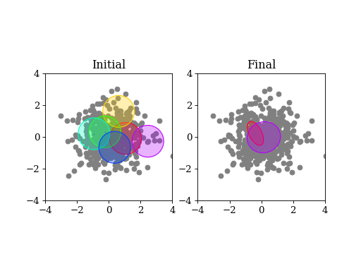
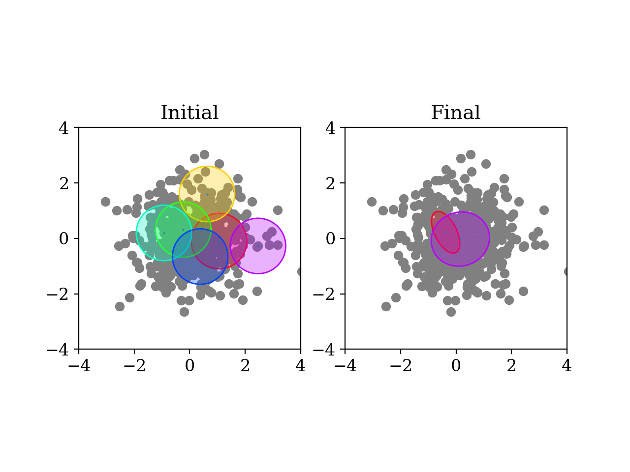
A basic example: draw samples from a standard Gaussian in 2D. Then run variational Bayes to recover that exact Gaussian. Paste the following code into your python shell and you should get plots similar to those shown modulo the random data points:

import numpy as np
from pypmc.mix_adapt.variational import GaussianInference
from pypmc.tools import plot_mixture
import matplotlib.pyplot as plt

# data points
N = 500
data = np.random.normal(size=2*N).reshape(N, 2)
# maximum number of components in mixture
K = 6
vb = GaussianInference(data, components=K,
                       alpha=10*np.ones(K),
                       nu=3*np.ones(K))

# plot data and initial guess
plt.subplot(1, 2, 1)
plt.scatter(data[:, 0], data[:, 1], color='gray')
initial_mix = vb.make_mixture()
plot_mixture(initial_mix, cmap='gist_rainbow')
x_range = (-4, 4)
y_range = x_range
plt.xlim(x_range)
plt.ylim(y_range)
plt.gca().set_aspect('equal')
plt.title('Initial')

# compute variational Bayes posterior
vb.run(prune=0.5*len(data) / K, verbose=True)

# obtain most probable mixture and plot it
mix = vb.make_mixture()
plt.subplot(1, 2, 2)
plt.scatter(data[:, 0], data[:, 1], color='gray')
plt.xlim(x_range)
plt.ylim(y_range)
plt.gca().set_aspect('equal')
plot_mixture(mix, cmap='gist_rainbow')
plt.title('Final')
plt.show()

(Source code, png, hires.png, pdf)

3.6.1.1. Initialization

In more complicated examples, it may be necessary to give good starting values to the means and covariances of the components in order to accelerate convergence to a sensible solution. You can pass this information when you create the GaussianInference object. Internally, the info is forwarded to a call to set_variational_parameters, where all parameter names and symbols are explained in detail.

If an initial guess in the form of a Gaussian MixtureDensity is available, this can be used to define the initial values using GaussianInference(... initial_guess=mixture)

Note that the vb object carries the posterior distribution of hyperparameters describing a Gaussian mixture. Invoking make_mixture() singles out the mixture at the mode of the posterior. To have a well defined mode one needs nu[k] > d and alpha[k] > 0 for at least one component k. We set \(\nu=3\) such that the covariance at the mode of the Wishart distribution

\[\boldsymbol{\Sigma} = (\nu - d) \boldsymbol{W}^{-1} = \boldsymbol{W}^{-1}\]

equals \(\boldsymbol{W}^{-1}\) for \(d=2\). This allows us to plot the initial guess. The default placement GaussianInference(...initial_guess="random") is to randomly select K data points and start with a Gaussian of unit covariance there. K is the maximum number of components and has to be chosen by user. A safe procedure is to choose K larger than desired, and let variational Bayes figures out the right value.

3.6.1.2. Running

Running variational Bayes with vb.run() can take a while if you have a lot of data points, lots of components, and high-dimensional data. Monitor the progress with verbose=True.

The pruning (removal) of components is determined by the prune keyword. After a VB update, every component is responsible for an effective number of samples. If this is lower than the threshold set by prune, the component is pruned. In our experiments, a good rule of thumb to remove many components is to set the threshold to \(K/2\).

3.6.1.3. Results

Continuing the example, you can inspect how all hyperparameters were updated by the data:

vb.prior_posterior()

and you can check that the mean of the most probable Gaussian (assuming the mixture only has one component) is close to zero and the covariance is close to the identity matrix:

mix = vb.make_mixture()
mix.components[0].mu
mix.components[0].sigma

3.7. Mixture reduction

Let us suppose samples are fed into a clustering algorithm that yields a Gaussian mixture. To save memory, we discard the samples and retain only the mixture as a description of the data. Assume the same procedure is carried out on different sets of samples from the same parent distribution, and we end up with a collection of mixture densities that contain similar information. How to combine them? A simple merge would be overly complex, as similar information is stored in every mixture. How then to compress this collection into one Gaussian mixture with less components but similar descriptive power? We provide two algorithms for this task illustrated in the example Mixture reduction.

3.7.1. Hierarchical clustering

While the KL divergence between two Gaussians is known analytically, the corresponding result between Gaussian mixtures is not known. The hierarchical clustering described in [GR04] seeks to minimize an ad-hoc function used as a proxy for the metric between two Gaussian mixtures. The basic idea is very simple: map input components to output components such that every component in the output mixture is made up of an integer number of input components (regroup step). Then update the output component weights, means, and covariances (refit step). Continue until the metric is unchanged.

Note that this is a discrete problem: each input component is associated to only one output component, thus if the mapping doesn’t change, then the metric does not change either. Output components can only die out if they receive no input component. Typically this is rare, so the number of output components is essentially chosen by the user, and not by the algorithm Hierarchical. A user has to supply the input mixture, and an initial guess of the output mixture, thereby defining the maximum number of components:

from pypmc.mix_adapt.hierarchical import Hierarchical

h = Hierarchical(input_mixture, initial_guess)

where both arguments are pypmc.density.mixture.MixtureDensity objects. To perform the clustering:

h.run()

Optional arguments to pypmc.density.mixture.MixtureDensity.run are the tolerance by which the metric may change to declare convergence (eps), whether to remove output components with zero weight (kill), and the total number of (regroup + refit) steps (max_steps).

3.7.2. VBmerge

In [BGP10], a variational algorithm is derived in the limit of large \(N\), the total number of virtual input samples. That is, the original samples are not required, only the mixtures. Hence the clustering is much faster but less accurate compared to standard variational Bayes. To create a VBMerge object, the required inputs are a MixtureDensity, the total number of samples encoded in the mixture \(N\), and the the maximum number of components \(K\) desired in the compressed output mixture:

from pypmc.mix_adapt.variational import VBMerge

VBMerge(input_mixture, N, K)

As guidance, if \(N\) is not known, one should choose a large number like \(N=10^4\) to obtain decent results.

The classes VBMerge and GaussianInference share the same interface; please check Classic version.

The great advantage compared to hierarchical clustering is that the number of output components is chosen automatically. One starts with (too) many components, updates, and removes those components with small weight using the prune argument to pypmc.mix_adapt.variational.GaussianInference.run.

3.8. Putting it all together

The examples in the next section show how to use the different algorithms in practice. The most advanced example, MCMC + variational Bayes, demonstrates how to combine various algorithms to integrate and sample from a multimodal function:

run multiple Markov chains to learn the local features of the target density;

combine the samples into a mixture density with variational Bayes

run importance sampling

rerun variational Bayes on importance samples

repeat importance sampling with improved proposal

combine samples with the deterministic-mixture approach