4. Examples
The following examples are available in a checkout of the repository
in the examples/ directory.
4.1. MCMC
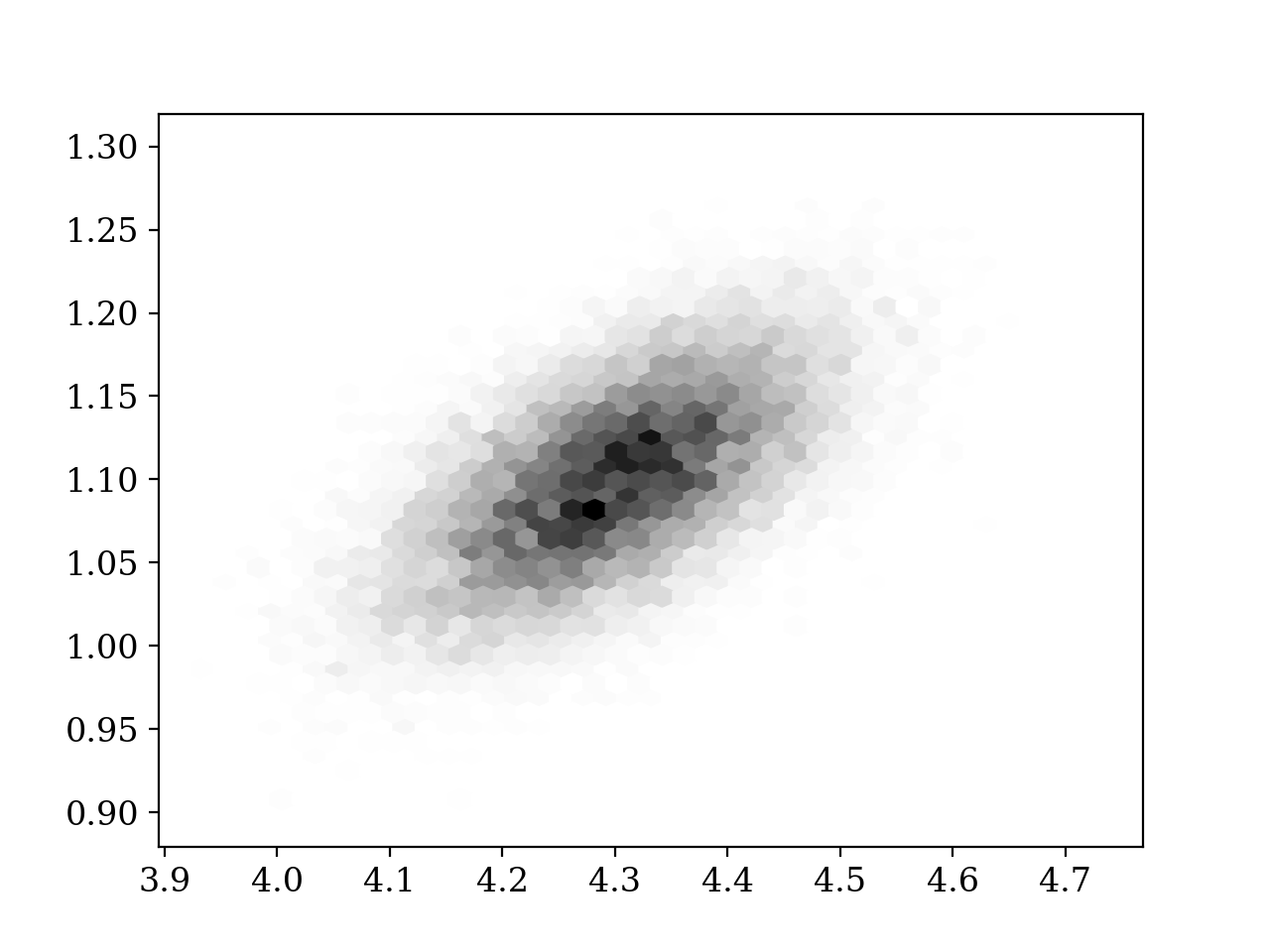
'''This example illustrates how to run a Markov Chain using pypmc'''

import numpy as np
import pypmc

# define a proposal
prop_dof   = 1.
prop_sigma = np.array([[0.1 , 0.  ]
                      ,[0.  , 0.02]])
prop = pypmc.density.student_t.LocalStudentT(prop_sigma, prop_dof)

# define the target; i.e., the function you want to sample from.
# In this case, it is a Gaussian with mean "target_mean" and
# covariance "target_sigma".
#
# Note that the target function "log_target" returns the log of the
# unnormalized gaussian density.
target_sigma = np.array([[0.01 , 0.003 ]
                        ,[0.003, 0.0025]])
inv_target_sigma = np.linalg.inv(target_sigma)
target_mean  = np.array([4.3, 1.1])

def unnormalized_log_pdf_gauss(x, mu, inv_sigma):
    diff = x - mu
    return -0.5 * diff.dot(inv_sigma).dot(diff)

log_target = lambda x: unnormalized_log_pdf_gauss(x, target_mean, inv_target_sigma)

# choose a bad initialization
start = np.array([-2., 10.])

# define the markov chain object
mc = pypmc.sampler.markov_chain.AdaptiveMarkovChain(log_target, prop, start)

# run burn-in
mc.run(10**4)

# delete burn-in from samples
mc.clear()

# run 100,000 steps adapting the proposal every 500 steps
# hereby save the accept count which is returned by mc.run
accept_count = 0
for i in range(200):
    accept_count += mc.run(500)
    mc.adapt()

# extract a reference to the history of all visited points
values = mc.samples[:]
accept_rate = float(accept_count) / len(values)
print("The chain accepted %4.2f%% of the proposed points" % (accept_rate * 100) )

# plot the result
try:
    import matplotlib.pyplot as plt
except ImportError:
    print('For plotting "matplotlib" needs to be installed')
    exit(1)

plt.hexbin(values[:,0], values[:,1], gridsize = 40, cmap='gray_r')
plt.show()
(Source code, png, hires.png, pdf)

4.2. PMC
4.2.1. Serial
'''This example shows how to use importance sampling and how to
adapt the proposal density using the pmc algorithm.
'''
import numpy as np
import pypmc
# define the target; i.e., the function you want to sample from.
# In this case, it is a bimodal Gaussian
#
# Note that the target function "log_target" returns the log of the
# target function.
component_weights = np.array([0.3, 0.7])
mean0 = np.array ([ 5.0 , 0.01 ])
covariance0 = np.array([[ 0.01 , 0.003 ],
[ 0.003, 0.0025]])
inv_covariance0 = np.linalg.inv(covariance0)
mean1 = np.array ([-4.0 , 1.0 ])
covariance1 = np.array([[ 0.1 , 0. ],
[ 0. , 0.02 ]])
inv_covariance1 = np.linalg.inv(covariance1)
component_means = [mean0, mean1]
component_covariances = [covariance0, covariance1]
target_mixture = pypmc.density.mixture.create_gaussian_mixture(component_means, component_covariances, component_weights)
log_target = target_mixture.evaluate
# define the initial proposal density
# In this case a three-modal gaussian used
# the initial covariances are set to the unit-matrix
# the initial component weights are set equal
initial_prop_means = []
initial_prop_means.append( np.array([ 4.0, 0.0]) )
initial_prop_means.append( np.array([-5.0, 0.0]) )
initial_prop_means.append( np.array([ 0.0, 0.0]) )
initial_prop_covariance = np.eye(2)
initial_prop_components = []
for i in range(3):
initial_prop_components.append(pypmc.density.gauss.Gauss(initial_prop_means[i], initial_prop_covariance))
initial_proposal = pypmc.density.mixture.MixtureDensity(initial_prop_components)
# define an ImportanceSampler object
sampler = pypmc.sampler.importance_sampling.ImportanceSampler(log_target, initial_proposal)
# draw 10,000 samples adapting the proposal every 1,000 samples
# hereby save the generating proposal component for each sample which is
# returned by sampler.run
# Note: With too few samples components may die out, and one mode might be lost.
generating_components = []
for i in range(10):
print("\rstep", i, "...\n\t", end='')
# draw 1,000 samples and save the generating component
generating_components.append(sampler.run(10**3, trace_sort=True))
# get a reference to the weights and samples that have just been generated
samples = sampler.samples[-1]
weights = sampler.weights[-1][:,0]
# update the proposal using the pmc algorithm in the non Rao-Blackwellized form
pypmc.mix_adapt.pmc.gaussian_pmc(samples, sampler.proposal, weights, generating_components[-1],
mincount=20, rb=True, copy=False)
print("\rsampling finished")
print( '-----------------')
print('\n')
# print information about the adapted proposal
print('initial component weights:', initial_proposal.weights)
print('final component weights:', sampler.proposal.weights)
print('target component weights:', component_weights)
print()
for k, m in enumerate([mean0, mean1, None]):
print('initial mean of component %i:' %k, initial_proposal.components[k].mu)
print('final mean of component %i:' %k, sampler.proposal.components[k].mu)
print('target mean of component %i:' %k, m)
print()
print()
for k, c in enumerate([covariance0, covariance1, None]):
print('initial covariance of component %i:\n' %k, initial_proposal.components[k].sigma, sep='')
print()
print('final covariance of component %i:\n' %k, sampler.proposal.components[k].sigma, sep='')
print()
print('target covariance of component %i:\n' %k, c, sep='')
print('\n')
# plot results
try:
import matplotlib.pyplot as plt
except ImportError:
print('For plotting "matplotlib" needs to be installed')
exit(1)
def set_axlimits():
plt.xlim(-6.0, +6.000)
plt.ylim(-0.2, +1.401)
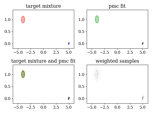
plt.subplot(221)
plt.title('target mixture')
pypmc.tools.plot_mixture(target_mixture, cmap='jet')
set_axlimits()
plt.subplot(222)
plt.title('pmc fit')
pypmc.tools.plot_mixture(sampler.proposal, cmap='nipy_spectral', cutoff=0.01)
set_axlimits()
plt.subplot(223)
plt.title('target mixture and pmc fit')
pypmc.tools.plot_mixture(target_mixture, cmap='jet')
pypmc.tools.plot_mixture(sampler.proposal, cmap='nipy_spectral', cutoff=0.01)
set_axlimits()
plt.subplot(224)
plt.title('weighted samples')
plt.hist2d(sampler.samples[-1][:,0], sampler.samples[-1][:,1], weights=sampler.weights[-1][:,0], cmap='gray_r', bins=200)
set_axlimits()
plt.tight_layout()
plt.show()
(Source code, png, hires.png, pdf)

4.2.2. Parallel
'''This example shows how to use importance sampling and how to
adapt the proposal density using the pmc algorithm in an MPI
parallel environment.
In order to have a multiprocessing enviroment invoke this script with
"mpirun -n 10 python pmc_mpi.py".

'''


from mpi4py.MPI import COMM_WORLD as comm

import numpy as np
import pypmc
import pypmc.tools.parallel_sampler # this submodule is NOT imported by ``import pypmc``

# This script is a parallelized version of the PMC example ``pmc.py``.
# The following lines just define a target density and an initial proposal.
# These steps are exactly the same as in ``pmc.py``:

# define the target; i.e., the function you want to sample from.
# In this case, it is a bimodal Gaussian
#
# Note that the target function "log_target" returns the log of the
# target function.
component_weights = np.array([0.3, 0.7])

mean0       = np.array ([ 5.0  , 0.01  ])
covariance0 = np.array([[ 0.01 , 0.003 ],
                        [ 0.003, 0.0025]])
inv_covariance0 = np.linalg.inv(covariance0)

mean1       = np.array ([-4.0  , 1.0   ])
covariance1 = np.array([[ 0.1  , 0.    ],
                        [ 0.   , 0.02  ]])
inv_covariance1 = np.linalg.inv(covariance1)

component_means = [mean0, mean1]
component_covariances = [covariance0, covariance1]

target_mixture = pypmc.density.mixture.create_gaussian_mixture(component_means, component_covariances, component_weights)

log_target = target_mixture.evaluate


# define the initial proposal density
# In this case it has three Gaussians:
# the initial covariances are set to the unit-matrix,
# the initial component weights are set equal
initial_prop_means = []
initial_prop_means.append( np.array([ 4.0, 0.0]) )
initial_prop_means.append( np.array([-5.0, 0.0]) )
initial_prop_means.append( np.array([ 0.0, 0.0]) )
initial_prop_covariance = np.eye(2)

initial_prop_components = []
for i in range(3):
    initial_prop_components.append(pypmc.density.gauss.Gauss(initial_prop_means[i], initial_prop_covariance))

initial_proposal = pypmc.density.mixture.MixtureDensity(initial_prop_components)

# -----------------------------------------------------------------------------------------------------------------------

# In ``pmc.py`` the following line defines the sequential single process sampler:
# sampler = pypmc.sampler.importance_sampling.ImportanceSampler(log_target, initial_proposal)
#
# We now use the parallel MPISampler instead:
SequentialIS = pypmc.sampler.importance_sampling.ImportanceSampler
parallel_sampler = pypmc.tools.parallel_sampler.MPISampler(SequentialIS, target=log_target, proposal=initial_proposal)

# Draw 10,000 samples adapting the proposal every 1,000 samples:

# make sure that every process has a different random number generator seed
if comm.Get_rank() == 0:
    seed = np.random.randint(1e5)
else:
    seed = None
seed = comm.bcast(seed)
np.random.seed(seed + comm.Get_rank())

generating_components = []
for i in range(10):
    # With the invocation "mpirun -n 10 python pmc_mpi.py", there are
    # 10 processes which means in order to draw 1,000 samples
    # ``parallel_sampler.run(1000//comm.Get_size())`` makes each process draw
    # 100 samples.
    # Hereby the generating proposal component for each sample in each process
    # is returned by ``parallel_sampler.run``.
    # In the master process, ``parallel_sampler.run`` is a list containing the
    # return values of the sequential ``run`` method of every process.
    # In all other processes, ``parallel_sampler.run`` returns the generating
    # component for its own samples only.
    last_generating_components = parallel_sampler.run(1000//comm.Get_size(), trace_sort=True)

    # In addition to the generating components, the ``sampler.run``
    # method automatically sends all samples to the master
    # process i.e. the process which fulfills comm.Get_rank() == 0.
    if comm.Get_rank() == 0:
        print("\rstep", i, "...\n\t", end='')

        # Now let PMC run only in the master process:

        # ``sampler.samples_list`` and ``sampler.weights_list`` store the weighted samples
        # sorted by the resposible process:
        # The History objects that are held by process i can be accessed via
        # ``sampler.<samples/weights>_list[i]``. The master process (i=0) also produces samples.

        # Combine the weights and samples to two arrays of 1,000 samples
        samples = np.vstack([history_item[-1] for history_item in parallel_sampler.samples_list])
        weights = np.vstack([history_item[-1] for history_item in parallel_sampler.weights_list])[:,0]

        # The latent variables are stored in ``last_generating_components``.
        # ``last_generating_components[i]`` returns an array with the generating
        # components of the samples produced by process number "i".
        # ``np.hstack(last_generating_components)`` combines the generating components
        # from all processes to one array holding all 1,000 entries.
        generating_components.append(  np.hstack(last_generating_components)  )

        # adapt the proposal using the samples from all processes
        new_proposal =  pypmc.mix_adapt.pmc.gaussian_pmc(samples, parallel_sampler.sampler.proposal,
                                                         weights, generating_components[-1],
                                                         mincount=20, rb=True)
    else:
        # In order to broadcast the ``new_proposal``, define a dummy variable in the other processes
        # see "MPI4Py tutorial", section "Collective Communication": http://mpi4py.scipy.org/docs/usrman/tutorial.html
        new_proposal = None

    # broadcast the ``new_proposal``
    new_proposal = comm.bcast(new_proposal)

    # replace the old proposal
    parallel_sampler.sampler.proposal = new_proposal

# only the master process shall print out any final information
if comm.Get_rank() == 0:
    all_samples  = np.vstack([history_item[ :] for history_item in parallel_sampler.samples_list])
    all_weights  = np.vstack([history_item[ :] for history_item in parallel_sampler.weights_list])
    last_samples = np.vstack([history_item[-1] for history_item in parallel_sampler.samples_list])
    last_weights = np.vstack([history_item[-1] for history_item in parallel_sampler.weights_list])
    print("\rsampling finished", end=', ')
    print("collected " + str(len(all_samples)) + " samples")
    print(  '------------------------------------------')
    print('\n')

    # print information about the adapted proposal
    print('initial component weights:', initial_proposal.weights)
    print('final   component weights:', parallel_sampler.sampler.proposal.weights)
    print('target  component weights:', component_weights)
    print()
    for k, m in enumerate([mean0, mean1, None]):
        print('initial mean of component %i:' %k, initial_proposal.components[k].mu)
        print('final   mean of component %i:' %k, parallel_sampler.sampler.proposal.components[k].mu)
        print('target  mean of component %i:' %k, m)
        print()
    print()
    for k, c in enumerate([covariance0, covariance1, None]):
        print('initial covariance of component %i:\n' %k, initial_proposal.components[k].sigma, sep='')
        print()
        print('final   covariance of component %i:\n' %k, parallel_sampler.sampler.proposal.components[k].sigma, sep='')
        print()
        print('target  covariance of component %i:\n' %k, c, sep='')
        print('\n')

    if comm.Get_size() == 1:
        print('******************************************************')
        print('********** NOTE: There is only one process. **********')
        print('******** try "mpirun -n 10 python pmc_mpi.py" ********')
        print('******************************************************')

    # plot results
    try:
        import matplotlib.pyplot as plt
    except ImportError:
        print('For plotting "matplotlib" needs to be installed')
        exit(1)

    def set_axlimits():
        plt.xlim(-6.0, +6.000)
        plt.ylim(-0.2, +1.401)

    plt.subplot(221)
    plt.title('target mixture')
    pypmc.tools.plot_mixture(target_mixture, cmap='jet')
    set_axlimits()

    plt.subplot(222)
    plt.title('pmc fit')
    pypmc.tools.plot_mixture(parallel_sampler.sampler.proposal, cmap='nipy_spectral', cutoff=0.01)
    set_axlimits()

    plt.subplot(223)
    plt.title('target mixture and pmc fit')
    pypmc.tools.plot_mixture(target_mixture, cmap='jet')
    pypmc.tools.plot_mixture(parallel_sampler.sampler.proposal, cmap='nipy_spectral', cutoff=0.01)
    set_axlimits()

    plt.subplot(224)
    plt.title('weighted samples')
    plt.hist2d(last_samples[:,0], last_samples[:,1], weights=last_weights[:,0], cmap='gray_r', bins=200)
    set_axlimits()

    plt.tight_layout()
    plt.show()
(Source code, png, hires.png, pdf)
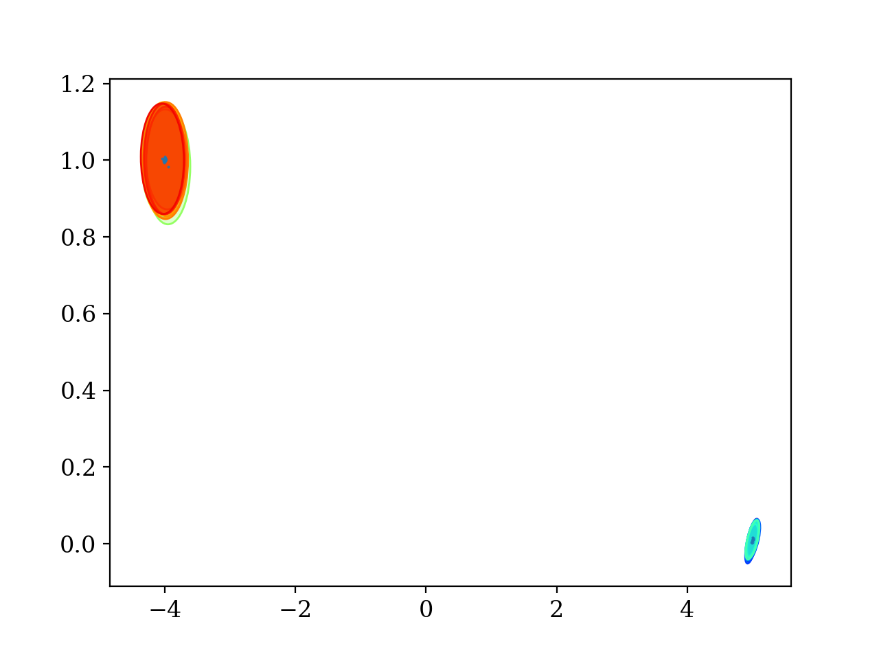
4.3. Grouping by Gelman-Rubin R value
'''This example illustrates how to group Markov Chains according to the
Gelman-Rubin R value (see [GR92]_).

'''

import numpy as np
import pypmc

# A Markov Chain can only explore a local mode of the target function.
# The Gelman-Rubin R value can be used to determine whether N chains
# explored the same mode. Pypmc offers a function which groups chains
# with a common R value less than some ``critical_r``.
#
# In this example, we run five Markov Chains initialized in different
# modes and then group those chains together that explored same mode.


# define a proposal
# this defines the same initial proposal for all chains
prop_dof   = 50.
prop_sigma = np.array([[0.1 , 0.  ]
                      ,[0.  , 0.02]])
prop = pypmc.density.student_t.LocalStudentT(prop_sigma, prop_dof)


# define the target; i.e., the function you want to sample from.
# In this case, it is a bimodal Gaussian with well separated modes.
#
# Note that the target function "log_target" returns the log of the
# target function.
component_weights = np.array([0.3, 0.7])

mean0       = np.array ([ 5.0  , 0.01  ])
covariance0 = np.array([[ 0.01 , 0.003 ],
                        [ 0.003, 0.0025]])
inv_covariance0 = np.linalg.inv(covariance0)

mean1       = np.array ([-4.0  , 1.0   ])
covariance1 = np.array([[ 0.1  , 0.    ],
                        [ 0.   , 0.02  ]])
inv_covariance1 = np.linalg.inv(covariance1)

component_means = [mean0, mean1]
component_covariances = [covariance0, covariance1]

target_mixture = pypmc.density.mixture.create_gaussian_mixture(component_means, component_covariances, component_weights)

log_target = target_mixture.evaluate

# choose initializations for the chains
# Here we place two chains into the mode at [5, 0.01] and three into the mode at [-4,1].
# In such a setup, the chains will only explore the mode where they are initialized.
# Different random numbers are used in each chain.
starts = [np.array([4.999, 0.])] * 2   +   [np.array([-4.0001, 0.999])] * 3

# define the markov chain objects
mcs = [pypmc.sampler.markov_chain.AdaptiveMarkovChain(log_target, prop, start) for start in starts]

# run and discard burn-in
for mc in mcs:
    mc.run(10**2)
    mc.clear()

# run 10,000 steps adapting the proposal every 500 steps
for mc in mcs:
    for i in range(20):
        mc.run(500)
        mc.adapt()

# extract a reference to the samples from all chains
stacked_values = [mc.samples[:] for mc in mcs]

# find the chain groups
# chains 0 and 1 are initialized in the same mode (at [5, 0.01])
# chains 2, 3 and 4 are initialized in the same mode (at [-4, 0])
# expect chain groups:
expected_groups = [[0,1], [2,3,4]]

# R value calculation only needs the means, variances (diagonal
# elements of covariance matrix) and number of samples,
# axis=0 ensures that we get variances separately for each parameter.
# critical_r can be set manually, here the default value is used
found_groups = pypmc.mix_adapt.r_value.r_group([np.mean(chain, axis=0) for chain in stacked_values],
                                               [np.var (chain, axis=0) for chain in stacked_values],
                                               len(stacked_values[0]))

# print the result
print("Expect %s" % expected_groups)
print("Have   %s"    % found_groups)

# Hint: ``stacked_values`` is an example of what `pypmc.mix_adapt.r_value.make_r_gaussmix()` expects as ``data``
result = pypmc.mix_adapt.r_value.make_r_gaussmix(stacked_values)

try:
    import matplotlib.pyplot as plt
except ImportError:
    print('For plotting "matplotlib" needs to be installed')
    exit(1)

pypmc.tools.plot_mixture(result, cmap='jet')
plt.show()
(Source code, png, hires.png, pdf)

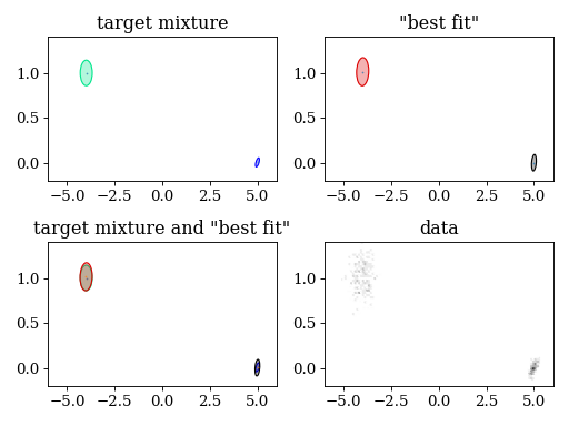
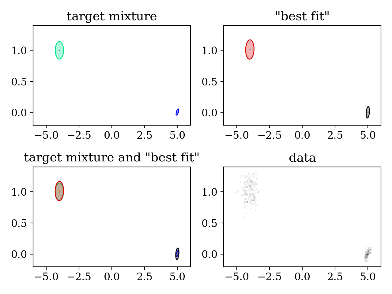
4.4. Variational Bayes
'''This example shows how to generate a "best fit" Gaussian mixture density
from data using variational Bayes.

'''

## in this example, we will:
## 1. Define a Gaussian mixture
## 2. Generate demo data from that Gaussian mixture
## 3. Generate a Gaussian mixture out of the data
## 4. Plot the original and the generated mixture


import numpy as np
import pypmc


# -------------------- 1. Define a Gaussian mixture --------------------

component_weights = np.array([0.3, 0.7])

mean0       = np.array ([ 5.0  , 0.01  ])
covariance0 = np.array([[ 0.01 , 0.003 ],
                        [ 0.003, 0.0025]])

mean1       = np.array ([-4.0  , 1.0   ])
covariance1 = np.array([[ 0.1  , 0.    ],
                        [ 0.   , 0.02  ]])

component_means = [mean0, mean1]
component_covariances = [covariance0, covariance1]

target_mix = pypmc.density.mixture.create_gaussian_mixture(component_means, component_covariances, component_weights)


# -------------------- 2. Generate demo data ---------------------------

data = target_mix.propose(500)


# -------------------- 3. Adapt a Gaussian mixture ---------------------

# maximum number of components
K = 20

# Create a "GaussianInference" object.
# The following command passes just the two essential arguments to "GaussianInference":
# The ``data`` and a maximum number of ``components``.
# For reasonable results in more complicated settings, a careful choice for ``W0``
# is crucial. As a rule of thumb, choose ``inv(W0)`` much smaller than the expected
# covariance. In this case, however, the default (``W0`` = unit matrix) is good enough.
vb = pypmc.mix_adapt.variational.GaussianInference(data, K)

# adapt the variational parameters
converged = vb.run(100, verbose=True)
print('-----------------------------')

# generate a Gaussian mixture with the most probable parameters
fit_mixture = vb.make_mixture()


# -------------------- 4. Plot/print results ---------------------------

if converged is None:
    print('\nThe adaptation did not converge.\n')
else:
    print('\nConverged after %i iterations.\n' %converged)

print("final  component weights: " + str(fit_mixture.weights))
print("target component weights: " + str( target_mix.weights))

try:
    import matplotlib.pyplot as plt
except ImportError:
    print('For plotting "matplotlib" needs to be installed')
    exit(1)

def set_axlimits():
    plt.xlim(-6.0, +6.000)
    plt.ylim(-0.2, +1.401)

plt.subplot(221)
plt.title('target mixture')
pypmc.tools.plot_mixture(target_mix, cmap='winter')
set_axlimits()

plt.subplot(222)
plt.title('"best fit"')
pypmc.tools.plot_mixture(fit_mixture, cmap='nipy_spectral')
set_axlimits()

plt.subplot(223)
plt.title('target mixture and "best fit"')
pypmc.tools.plot_mixture(target_mix, cmap='winter')
pypmc.tools.plot_mixture(fit_mixture, cmap='nipy_spectral')
set_axlimits()

plt.subplot(224)
plt.title('data')
plt.hexbin(data[:,0], data[:,1], cmap='gray_r')
set_axlimits()

plt.tight_layout()
plt.show()
(Source code, png, hires.png, pdf)

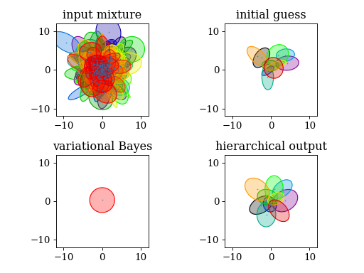
4.5. Mixture reduction
'''Demonstrate the usage of hierarchical clustering and variational
Bayes (VBMerge) to reduce a given Gaussian mixture to a Gaussian
mixture with a reduced number of components.

'''

import numpy as np
from scipy.stats import chi2
import pypmc

# dimension
D = 2

# number of components
K = 400

# Wishart parameters: mean W, degree of freedom nu
W = np.eye(D)
nu = 5

# "draw" covariance matrices from Wishart distribution
def wishart(nu, W):
    dim = W.shape[0]
    chol = np.linalg.cholesky(W)
    tmp = np.zeros((dim,dim))
    for i in range(dim):
        for j in range(i+1):
            if i == j:
                tmp[i,j] = np.sqrt(chi2.rvs(nu-(i+1)+1))
            else:
                tmp[i,j] = np.random.normal(0,1)
    return np.dot(chol, np.dot(tmp, np.dot(tmp.T, chol.T)))

covariances = [wishart(nu, W) for k in range(K)]

# put components at positions drawn from a Gaussian around mu
mu = np.zeros(D)
means = [np.random.multivariate_normal(mu, sigma) for sigma in covariances]

# equal weights for every component
weights = np.ones(K)

# weights are automatically normalized
input_mixture = pypmc.density.mixture.create_gaussian_mixture(means, covariances, weights)

# create initial guess from first K_out components
K_out = 10
initial_guess = pypmc.density.mixture.create_gaussian_mixture(means[:K_out], covariances[:K_out], weights[:K_out])

###
# hierarchical clustering
#
# - the output closely resembles the initial guess
# - components laid out spherically symmetric
# - every component is preserved
###
h = pypmc.mix_adapt.hierarchical.Hierarchical(input_mixture, initial_guess)
h.run(verbose=True)

###
# VBMerge
#
# - N is the number of samples that gave rise to the input mixture. It
#   is arbitrary, so play around with it. You might have to adjust the
#   ``prune`` parameter in the ``run()`` method
# - only one component survives, again it is spherically symmetric
###
vb = pypmc.mix_adapt.variational.VBMerge(input_mixture, N=1000,
                                         initial_guess=initial_guess)
print()
print("Start variational Bayes:")
vb.run(verbose=True)

# plot results
try:
    import matplotlib.pyplot as plt
except ImportError:
    print('For plotting "matplotlib" needs to be installed')
    exit(1)

def set_axlimits():
    plt.gca().set_aspect('equal')
    plt.xlim(-12.0, +12.0)
    plt.ylim(-12.0, +12.0)

plt.subplot(221)
plt.title('input mixture')
pypmc.tools.plot_mixture(input_mixture)
set_axlimits()

plt.subplot(222)
plt.title('initial guess')
pypmc.tools.plot_mixture(initial_guess)
set_axlimits()

plt.subplot(223)
plt.title('variational Bayes')
pypmc.tools.plot_mixture(vb.make_mixture(), cmap='autumn')
set_axlimits()

plt.subplot(224)
plt.title('hierarchical output')
pypmc.tools.plot_mixture(h.g)
set_axlimits()

plt.tight_layout()
plt.show()
(Source code, png, hires.png, pdf)
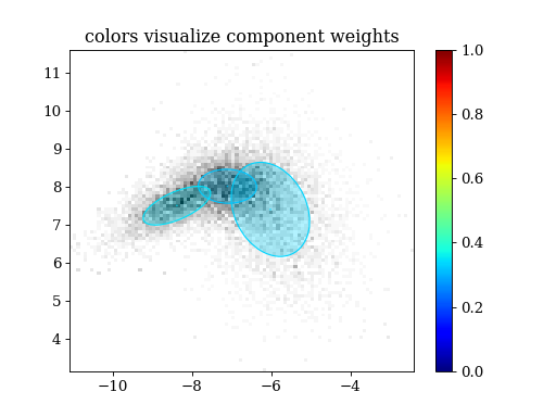
4.6. MCMC + variational Bayes
'''This example illustrates how pypmc can be used to integrate a
non-negative function. The presented algorithm needs very little
analytical knowledge about the function.

'''

import numpy as np
import pypmc

# The idea is to find a good proposal function for importance sampling
# with as little information about the target function as possible.
#
# In this example we will first map out regions of interest using Markov
# chains, then we use the variational Bayes to approximate the target
# with a Gaussian mixture.

# *************************** Important: ***************************
# * The target function must be defined such that it returns the   *
# * log of the function of interest. The methods we use imply that *
# * the function is interpreted as an unnormalized probability     *
# * density.                                                       *
# ******************************************************************

# Define the target; i.e., the function you want to sample from.  In
# this case, it is a Student's t mixture of three components with
# different degrees of freedom. They are located close to each other.
# If you want a multimodal target, adjust the means.

dim = 2

mean0       = np.array ([-6.0,  7.3  ])
covariance0 = np.array([[ 0.8, -0.3 ],
                        [-0.3,  1.25]])

mean1       = np.array ([-7.0,  8.0   ])
covariance1 = np.array([[ 0.5,  0.    ],
                        [ 0. ,  0.2  ]])

mean2       = np.array ([-8.5,  7.5   ])
covariance2 = np.array([[ 0.5,  0.2   ],
                        [ 0.2,  0.2  ]])

component_weights = np.array([0.3, 0.4, 0.3])
component_means = [mean0, mean1, mean2]
component_covariances = [covariance0, covariance1, covariance2]
dofs = [13, 17, 5]

target_mixture = pypmc.density.mixture.create_t_mixture(component_means, component_covariances, dofs, component_weights)
log_target = target_mixture.evaluate

# Now we suppose that we only have the following knowledge about the
# target function: its regions of interest are at a distance of no more
# than order ten from zero.

# Now we try to find these with Markov chains.  We have to deal with
# the fact that there may be modes separated by regions of very low
# probability. It is thus unlikely that a single chain explores more
# than one mode in such a case. To deal with this multimodality, we
# start several chains and hope that they find all modes.  We will
# start ten Markov chains at random positions in the square
# [(-10,-10), (+10,+10)].
starts = [np.random.uniform(-10,10, size=dim) for i in range(10)]

# For a local-random-walk Markov chain, we also need an initial
# proposal.  Here, we take a gaussian with initial covariance
# diag(1e-3).  The initial covariance should be chosen such that it is
# of the same order as the real covariance of the mode to be mapped
# out. For a Gaussian target, the overall scale should
# decrease as 2.38^2/d as the dimension d increases to achieve an
# acceptance rate around 20%.
mc_prop = pypmc.density.gauss.LocalGauss(np.eye(dim) * 2.38**2 / dim)
mcs = [pypmc.sampler.markov_chain.AdaptiveMarkovChain(log_target, mc_prop, start) for start in starts]

print('running Markov chains ...')

# In general we need to let the chain move to regions of high
# probability, these samples are not representative, so we discard them
# as burn-in. Then we let the Markov chains map out the regions of
# interest. The samples are used to adapt the proposal covariance to
# yield a satisfactory acceptance rate.
for mc in mcs:
    for i in range(20):
        mc.run(500)
        mc.adapt()
        if i == 0:
            mc.clear()

mc_samples_sorted_by_chain = [mc.samples[:] for mc in mcs]
mc_samples = np.vstack(mc_samples_sorted_by_chain)

means = np.zeros((len(mcs), dim))
variances = np.zeros_like(means)

for i,mc in enumerate(mc_samples_sorted_by_chain):
    means[i] = mc.mean(axis=0)
    variances[i] = mc.var(axis=0)

# Now we use the Markov chain samples to generate a mixture proposal
# function for importance sampling. For this purpose, we choose the
# variational Bayes algorithm that takes samples and an initial guess
# of the mixture as input. To create the initial guess, we group all
# chains that mixed, and create 10 components per group. For a
# unimodal target, all chains should mix. For more information about
# the following call, check the example "Grouping by Gelman-Rubin R
# value"(r-group.py) or the reference documentation.
long_patches = pypmc.mix_adapt.r_value.make_r_gaussmix(mc_samples_sorted_by_chain, K_g=10)

# Comments on arguments:
#   o mc_samples[::100]   - Samples in the Markov chains are strongly correlated
#                           => thin the samples to get approx. independent samples
#   o W0=np.eye(dim)*1e10 - The resulting covariance matrices can be very
#                           sensitive to W0. Its inverse should be chosen much
#                           smaller than the actual covariance. If it is too small,
#                           W0 will dominate the resulting covariances and
#                           usually lead to very bad results.
vb = pypmc.mix_adapt.variational.GaussianInference(mc_samples[::100], initial_guess=long_patches, W0=np.eye(dim)*1e10)

# When we run variational Bayes, we want unneccessary components to be
# automatically pruned. The prune parameter sets how many samples a
# component must effectively have to be considered important. The rule
# of thumb employed here proved good in our experiments.
vb_prune = 0.5 * len(vb.data) / vb.K

# Run the variational Bayes for at most 1,000 iterations.  But if the
# lower bound of the model evidence changes by less than `rel_tol`,
# convergence is declared before. If we increase `rel_tol` to 1e-4, it
# takes less iterations but potentially more (useless) components
# survive the pruning. The trade-off depends on the complexity of the
# problem.
print('running variational Bayes ...')
vb.run(1000, rel_tol=1e-8, abs_tol=1e-5, prune=vb_prune, verbose=True)

# extract the most probable Gaussian mixture given the samples
vbmix = vb.make_mixture()

# Now we can instantiate an importance sampler. We draw 1,000
# importance samples and use these for a proposal update using
# variational Bayes again. In case there are multiple modes and
# the chains did not mix, we need this step to infer the right
# component weights because the component weight is given by
# how many chains it attracted, which could be highly dependent
# on the starting points and independent of the correct
# probability mass.
print('running importance sampling ...')
sampler = pypmc.sampler.importance_sampling.ImportanceSampler(log_target, vbmix)
sampler.run(1000)

# The variational Bayes allows us, unlike PMC, to include the
# information gained by the Markov chains in subsequent proposal
# updates. We know that we cannot trust the component weights obtained
# by the chains. Nevertheless, we can rely on the means and covariances. The
# following lines show how to code that into the variational Bayes by
# removing the hyperparameter `alpha0` that encodes the component
# weights.
prior_for_proposal_update = vb.posterior2prior()
prior_for_proposal_update.pop('alpha0')
vb2 = pypmc.mix_adapt.variational.GaussianInference(sampler.samples[:],
                                                    initial_guess=vbmix,
                                                    weights=sampler.weights[:][:,0],
                                                    **prior_for_proposal_update)

# Note: This time we leave "prune" at the default value "1" because we
#       want to keep all components that are expected to contribute
#       with at least one effective sample per importance sampling run.
print('running variational Bayes ...')
vb2.run(1000, rel_tol=1e-8, abs_tol=1e-5, verbose=True)
vb2mix = vb2.make_mixture()

# Now we draw another 10,000 samples with the updated proposal
sampler.proposal = vb2mix
print('running importance sampling ...')
sampler.run(10**4)

# We can combine the samples and weights from the two runs, see reference [Cor+12].
weights = pypmc.sampler.importance_sampling.combine_weights([samples[:]      for samples in sampler.samples],
                                                            [weights[:][:,0] for weights in sampler.weights],
                                                            [vbmix, vb2mix]                                 ) \
                                                            [:][:,0]
samples = sampler.samples[:]

# The integral can then be estimated from the weights. The error is also
# estimated from the weights. By the central limit theorem, the integral
# estimator has a gaussian distribution.
integral_estimator = weights.sum() / len(weights)
integral_uncertainty_estimator = np.sqrt((weights**2).sum() / len(weights) - integral_estimator**2) / np.sqrt(len(weights)-1)

print('analytical integral = 1')
print('estimated  integral =', integral_estimator, '+-', integral_uncertainty_estimator)

# Let's see how good the proposal matches the target density: the closer
# the values of perplexity and effective sample size (ESS) are to 1,
# the better.  Outliers, or samples out in the tails of the target
# with a very large weight, show up in the 2D marginal and reduce the
# ESS significantly. For the above integral estimate to be right on
# average, they are 'needed'. Without outliers (most of the time), the
# integral is a tad too small.
print('perplexity', pypmc.tools.convergence.perp(weights))
print('effective sample size', pypmc.tools.convergence.ess(weights))

# As mentioned in the very beginning, the methods we applied reinterpret
# the target function as an unnormalized probability density.
# In addition to the integral, we also get weighted samples distributed according
# to that probability density.
try:
    import matplotlib.pyplot as plt
except ImportError:
    print('For plotting "matplotlib" needs to be installed')
    exit(1)

plt.figure()
plt.hist2d(samples[:,0], samples[:,1], weights=weights, bins=100, cmap='gray_r')
pypmc.tools.plot_mixture(sampler.proposal, visualize_weights=True, cmap='jet')
plt.colorbar()
plt.clim(0.0, 1.0)
plt.title('colors visualize component weights')
plt.show()
(Source code, png, hires.png, pdf)
